Deep Learning for Iterative Spectral CT Reconstruction: Replacing Statistical Iterations with an Attention-Based U-Net
Generating a phantom and a sinogram
Generate a phantom where each pixel consists of part bone and part water described as (bone, water)
Background values should be low for both to simulate air (0, 0.05)
main body should be elliptical and mainly consist of water (0.20, 0.80)
elliptical inserts should simulate different organs and/or body featurs (0.80, 0.80)
Generate a sinogram from the projections
The function will return a 3D object containing the sinograms for the height of the detector. We want to select a slice to display
print a 2D cross section of the phantom with a corresponding sinogram
#settings
objectSize = 32     # size of the object
nPixelsY = 64       # number of pixels in Y direction detector
nPixelsZ = 44       # number of pixels in Z direction detector
projections = 64    # number of projections
iterations = 40     # number of iterations
generate phantom
import random, numpy as np

def generate_phantom(n, h, num_features=1):

    h = random.randint(1, 3)  # Random height offset for the torso

    # Initialize 3D bone and water matrices with zeros
    bone_matrix = np.zeros((n, n, n), dtype=float)
    water_matrix = np.zeros((n, n, n), dtype=float)

    # fill background of matrices with 0.05 bone and water
    bone_matrix.fill(0.05)
    water_matrix.fill(0.05)

    # set values for main ellipse (simulated torso)
    intensity_bone = random.uniform(0.1, 0.6)
    intensity_water = random.uniform(0.1, 0.6)  # Random intensity for water

    offset_i = np.random.randint(-h, h + 1)
    offset_j = np.random.randint(-h, h + 1)

    center_i = n // 2 + offset_i
    center_j = n // 2 + offset_j

    # Main body ellipse (simulated torso with random offset)
    for i in range(h, n - h):
        for j in range(2 * h, n - 2 * h):
            if ((i - center_i) / ((n - 2 * h) / 2)) ** 2 + ((j - center_j) / ((n - 6 * h) / 2)) ** 2 <= 1:
                bone_matrix[2*h:-2*h, i, j] = intensity_bone
                water_matrix[2*h:-2*h, i, j] = intensity_water

    # Adding smaller features (e.g., organs or bone structures)
    for _ in range(num_features):

        # Random place in the body - h is the offset from the edge, n is the size of the matrix
        a = random.randint(h, (n - h) // 4)  # Semi-major axis
        b = random.randint(h, (n - h) // 4)  # Semi-minor axis
        center_x = random.randint(h + a, n - h - a)
        center_y = random.randint(3 * h + b, n - 3 * h - b)

        a_water = random.randint(h, (n - h) // 4)  # Semi-major axis for water
        b_water = random.randint(h, (n - h) // 4)  # Semi-minor axis for water

        # Randomly choose the intensity for bone and water, together they add to 1.
        bone_intensity = 0.8
        water_intensity = 0.8

        for i in range(center_x - a_water, center_x + a_water):
            for j in range(center_y - b_water, center_y + b_water):
                if 0 <= i < n and 0 <= j < n:
                    if ((i - center_x) / a_water) ** 2 + ((j - center_y) / b_water) ** 2 <= 1:
                        bone_matrix[2*h:-2*h, i, j] = bone_intensity

        center_x = random.randint(h + a, n - h - a)
        center_y = random.randint(3 * h + b, n - 3 * h - b)

        for i in range(center_x - a, center_x + a):
            for j in range(center_y - b, center_y + b):
                if 0 <= i < n and 0 <= j < n:
                    if ((i - center_x) / a) ** 2 + ((j - center_y) / b) ** 2 <= 1:
                        water_matrix[2*h:-2*h, i, j] = water_intensity

    water_matrix *= 1  # Water density is 1
    bone_matrix *= 1.92  # Apply bone density

    return bone_matrix, water_matrix

bone, water = generate_phantom(objectSize, 2, num_features=1)
x = np.column_stack((bone.ravel(), water.ravel()))

# show phantom for bone
plt.imshow(bone[objectSize // 2, :, :], cmap='gray')
plt.show()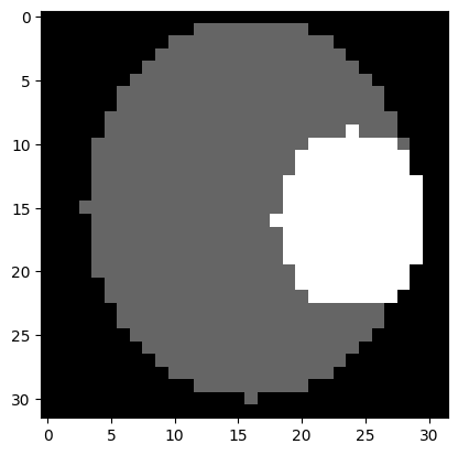
Running projection algorithm
from libs.simulatepreps import projectMatrix

#generate proection matrices
y, S, M, A = projectMatrix(x, objectSize, nPixelsY, nPixelsZ, 1, projections)
Generating sinogram
def getSinogram(y, energy_bin_index=0, z_index=32, nProj=100, detector_shape=(64, 44)):
    nX, nZ = detector_shape
    y_bin = y[energy_bin_index]
    y_proj_zx = y_bin.reshape((nProj, nZ, nX))  # shape: (100, 64, 44)
    sinogram = y_proj_zx[:, z_index, :]  # shape: (100, 44)
    return sinogram

sinogram = getSinogram(y, energy_bin_index=0, z_index=objectSize // 2, nProj=projections, detector_shape=(nPixelsY, nPixelsZ))
Make figure
import matplotlib.pyplot as plt


# plot bone density and phantom at objectSize //2
plt.figure(figsize=(12, 6))
plt.subplot(1, 2, 1)
plt.imshow(bone[objectSize // 2, :, :], cmap='gray')
plt.title('Bone Density at z = {}'.format(objectSize // 2))
plt.xlabel('X')
plt.ylabel('Y')

plt.subplot(1, 2, 2)
plt.imshow(sinogram, cmap='gray')
plt.title('Sinogram at z = {}'.format(objectSize // 2))
plt.ylabel('Angle')
plt.xlabel('Y')

plt.tight_layout()
plt.show()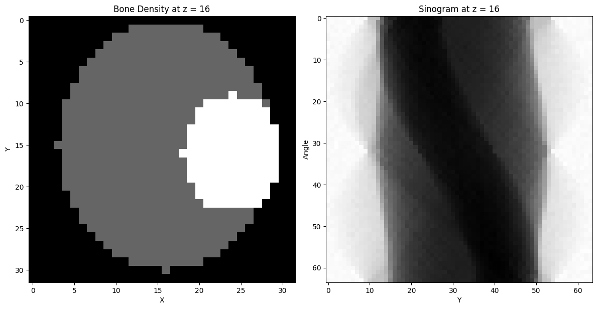
Visualising a 2D convolution
# we want to put the phantom through a pytorch 2d convolution layer
import torch

bone_array = bone[objectSize // 2, :, :]
bone_tensor = torch.tensor(bone[objectSize // 2, :, :], dtype=torch.float32)

# create a 2D convolution layer with a kernel size of 3x3
conv_layer = torch.nn.Conv2d(in_channels=1, out_channels=1, kernel_size=3, padding=1)

# apply the convolution layer to the bone tensor
output_tensor = conv_layer(bone_tensor.unsqueeze(0).unsqueeze(0))  # Add batch and channel dimensions
output_image = output_tensor.squeeze(0).squeeze(0).detach().numpy()  # Remove batch and channel dimensions

# plot 2 plots, one of the original bone image with a square showing one of the convolution kernels, and next to it the output image
plt.figure(figsize=(12, 6))
#make sure xlabel and ylabel are larger
plt.rcParams['axes.labelsize'] = 14
plt.subplot(1, 2, 1)
plt.imshow(bone_tensor.numpy(), cmap='gray')
# draw a square representing the convolution kernel
kernel_size = conv_layer.kernel_size[0]
plt.gca().add_patch(plt.Rectangle((10.5, 20.5), kernel_size, kernel_size, edgecolor='red', facecolor='none', lw=2))
# fill square with rectengles for each pixel
for i in range(kernel_size):
    for j in range(kernel_size):
        plt.gca().add_patch(plt.Rectangle((10.5 + i, 20.5 + j), 1, 1, edgecolor='red', facecolor='none', lw=0.5))
plt.xlabel('X')
plt.ylabel('Y')
plt.subplot(1, 2, 2)
plt.imshow(output_image, cmap='gray')
# draw little square representing the pixel on which the convolution was applied
plt.gca().add_patch(plt.Rectangle((10.5+2, 20.5+2), 1, 1, edgecolor='red', facecolor='none', lw=2))
plt.xlabel('X')
plt.ylabel('Y')
plt.show()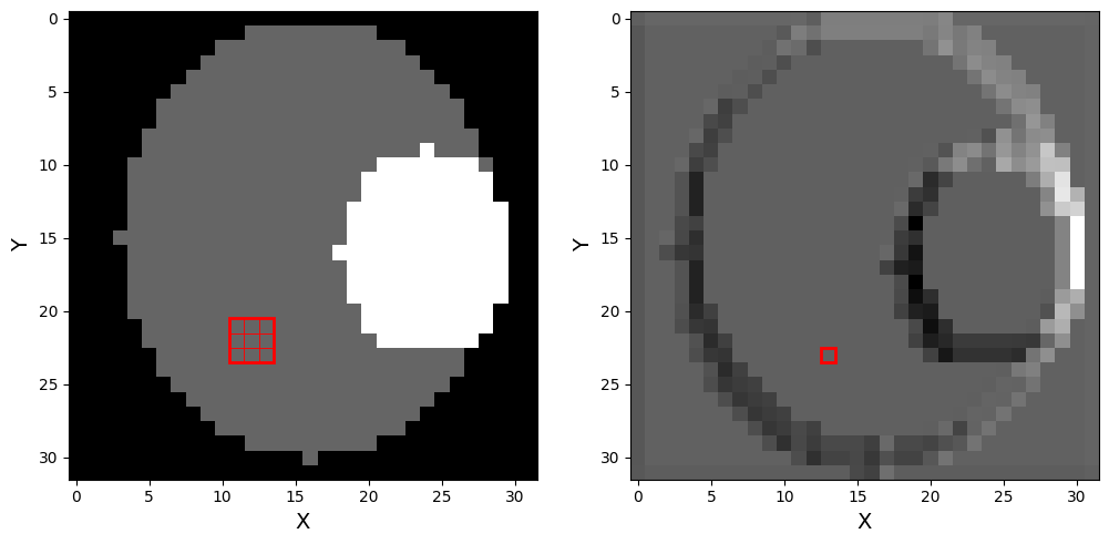
Deep Learning for Iterative Spectral CT Reconstruction: Replacing Statistical Iterations with an Attention-Based U-Net
Deep Learning for Iterative Spectral CT Reconstruction: Replacing Statistical Iterations with an Attention-Based U-NetDeep Learning for Iterative Spectral CT Reconstruction: Replacing Statistical Iterations with an Attention-Based U-Net
Reconstruction