Deep Learning for Iterative Spectral CT Reconstruction: Replacing Statistical Iterations with an Attention-Based U-Net
Author: Luuk Fröling
Abstract
In the past decade, spectral CT imaging has gained significant attention for its ability to differentiate between materials. Using photon counting detectors (PCD), individually measured x-ray photons can be sorted into energy bins. These energy-resolved measurements enable the reconstruction of material density images through iterative algorithms, providing detailed information about tissue composition. This study aims to accelerate the iterative reconstruction process by introducing a machine learning model. Specifically, an attention-based U-Net (AttU-Net) is trained to iteratively reconstruct material density images from spectral measurements. To achieve this goal, the model will be trained on the iterations of a pre-existing statistical iterative method. The network architecture consists of five convolutional layers in the encoder and five up-convolution layers in the decoder. Attention mechanisms are incorporated into the skip connections, where gating signals are derived from decoder feature maps. After 180 training epochs using 506 phantoms and 4,554 input-output sets, the AttU-Net is able to recognise the general structure of bone and water within the phantom images. However, it struggles to reliably differentiate between the two materials. While the model achieves a lower root-mean-squared (RMS) error than the iterative algorithm in the first iteration, and does so 1.30× faster, it ultimately converges to a higher final error. Subsequent iterations of the model do not provide a meaningful speedup, as the reconstruction error remains too high for practical use. To reduce the error, the training data must be filtered to ensure only high-quality examples are used for training.
Introduction
With the invention of the first viable computed tomography (CT) scanner by Godfrey Hounsfield in 1972, funded in part by sales from ‘the beatles’ records Pietzsch, 2025, the field of medical imaging gained the ability to produce cross-sectional images of the human body. CT images are generated by rotating an x-ray source and a detector around an object being scanned. The resulting images show, like regular x-ray images, how much radiation is absorbed per voxel (the attenuation coefficient). However, different materials may exhibit similar absorption properties, making it difficult to distinguish between them in conventional CT scans.
The introduction of photon counting detectors (PCD), which can detect individual photons and their energy Taguchi & Iwanczyk, 2013, makes it possible to exploit the energy dependence of the attenuation coefficient to differentiate these materials. By sorting the detected photons into discrete energy bins, multiple energy-selective measurements can be obtained. These spectral measurements enable the reconstruction of material-specific images through a process known as material decomposition.
Material decomposition requires advanced reconstruction algorithms to generate multiple images from the energy-selective measurements. These algorithms, iterative algorithm proposed by Mechlem et al., 2018, are often computationally heavy and time-consuming. If successfully implemented, spectral CT scan images provide in-depth information about the types of tissue present in an image.
Recent advances in machine learning and neural networks, particularly U-Nets Oktay et al., 2018 and attention mechanisms Vaswani et al., 2017, have shown great potential for image reconstruction tasks. Combining these techniques can allow a model to be capable of learning complex spatial relationships, where such a model has the potential to accelerate or replace traditional iterative methods.
In this work, an attention-based U-Net (AttU-Net) is employed to replace the steps of the iterative reconstruction algorithm. The input data consists of projections acquired using a PCD, which provides energy-dependent measurements by sorting the measured photon counts in energy-bins. Focusing on the material decomposition capabilities of dual-energy CT scans, the AttU-Net model is trained to iteratively reconstruct both water and bone density images based on training data taken from the iterative reconstruction algorithm described in Mechlem et al., 2018.
To train the model, simulated projection data is generated using phantoms consisting of a cylindrical body with two distinct regions: one with higher bone density and one with higher water density. After training the model on these phantoms, validation is performed using a separate set of 20 unseen phantoms. The reconstructed images are evaluated using root-mean-squared (RMS) error analysis and visual inspection. Additionally, a speedup metric is introduced to compare how fast the AttU-Net reaches a comparable RMS error to that of the iterative method.
Theory
Basics CT scans
A computed tomography (CT) scanner is an imaging device that uses x-rays to create cross-sectional images of an object. It consists of an x-ray source and a detector placed at a distance from each other. During scanning, both the source and the detector will rotate around the object to be imaged at several angles. For each step, the source emits x-rays that pass through the object and the transmitted photons are measured by the detector. The number of detected photons at position i along the detector for an ideal, noise-free measurement is given by:
where is the number of the x-rays emitted by the source and is the linear attenuation coefficient that depends on position and x-ray energy . The integral is taken along the path , which represents the trajectory of x-rays from the source to detector position . This accounts for the cumulative attenuation experienced by x-rays along their path through the object where describes how much of the incoming x-rays are absorbed per unit of length Kamalian et al., 2016.
By rotating the source and detector around the object and recording measurements at multiple angles, a sinogram can be created. A sinogram is a 2D plot where each column corresponds to a detector reading at a specific projection angle.
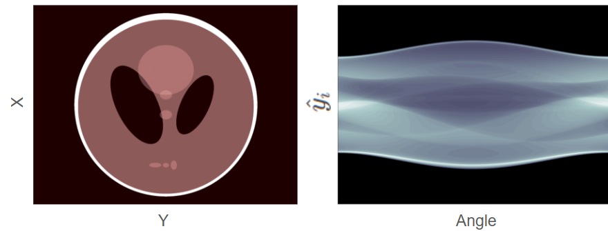
Figure 1:left: A phantom with multiple structures (ellipses) of different densities right corresponding sinogram. The darker regions in the sinogram indicate higher photon counts. Figure reproduced from Leuschner et al., 2019
A phantom and a corresponding sinogram can be seen in Figure 1. The phantom contains multiple, elliptical structures of different densities. On the right is the corresponding sinogram where the darker parts of the sinogram correspond to more detected photons.
Cone beam CT scan
The sinogram in Figure 1 is true for a 1D detector, where we construct a single slice. A cone beam CT scan uses a source emitting x-rays in a cone-beam shape, which can be detected on a 2D flat-panel detector Venkatesh & Elluru, 2017.
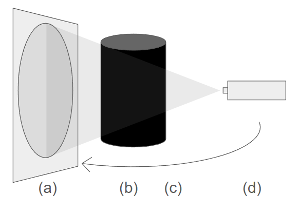
Figure 2:A schematic drawing of a cone-beam CT scan: (a) the 2D detector panel, (b) the phantom, (c) rotation direction of the source-detector pair (d) the x-ray source.
Figure 2 shows a cone beam CT scan setup, where both the detector and the source rotate around the object to acquire a set of 2D projection measurements at multiple angles. these measurements are known as projections and allow for a 3D image to be reconstructed.
The relationship between the object and the measured rays can be described by a projection matrix . This matrix has dimensions where is the number of voxels in the object and is the number of rays (measurements) collected by the detector. Each element of the matrix is the contribution of the voxel of the object to be imaged to the ray of the detector Yang et al., 2017. The measured projections can thus be modeled as:
where is the vectorised representation of the voxel values and contains the corresponding ray measurements. This formulation will be used by the reconstruction algorithms during the simulations. To better reflect the statistical fluctuations during photon detection, noise is applied to the computed projections. To simulate measurement noise, each ideal projection value is used as the mean of a Poisson distribution from which a noisy measurement is sampled.
Detector types
Currently, most CT scanners use an energy integrating detector (EID) Marth et al., 2023. An EID measures the intensity of the incoming x-rays by a two-step process: scintillation followed by photodetection. The scintillator absorbs the x-rays which have passed through the body and emits light in the visible spectrum. These re-emitted photons can be detected by photodetectors located underneath the scintillator. Due to the difference in energy of the incoming x-ray and the emitted visible light, multiple light photons can be re-emitted. To measure a signal, EIDs integrate over time which loses all energy dependent information Taguchi & Iwanczyk, 2013.
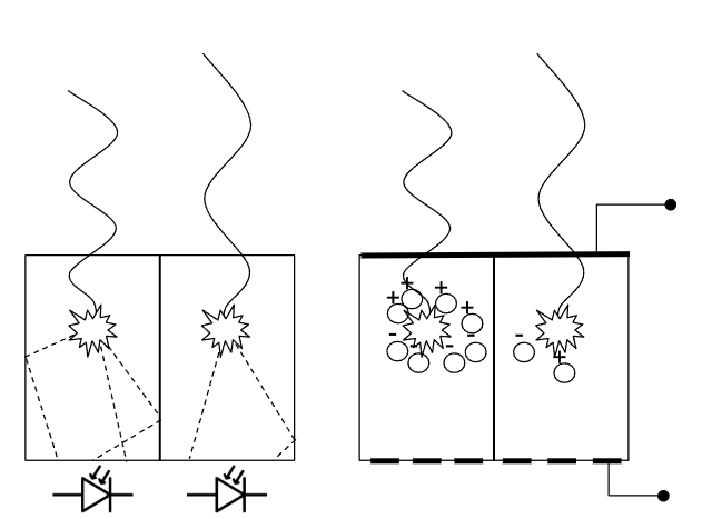
Figure 3:left: An EID where the incoming x-rays are absorbed within the scintillator. Several photons within the visible light spectrum are re-emitted which can be measured by the photodiodes located below the scintillator. right: A PCD where incoming x-rays create electron-hole pairs in a semiconductor. This creates a current between the top and bottom of the semiconductor which can be measured by electrodes, preserving energy dependent information.
Photon-counting detector (PCD) CT scans improve the measurements by directly transforming the incoming X-ray photons into an energy-dependent signal, as illustrated in Figure 3. In a PCD, each photon is absorbed in a semiconductor layer, generating electron-hole pairs that produce an electric signal proportional to the photon’s energy. Unlike EIDs, PCDs can measure the energy of individual photons.
Commonly available X-ray sources emit a polychromatic spectrum Antsiferov, 2003, meaning the emitted photons span a broad range of energies rather than a single energy level. The PCD measures the energy of the incoming photons and sorts these into multiple energy bins, each representing a specific range within the spectrum Taguchi et al., 2022. By comparing the counts across these energy bins, multiple energy-resolved measurements can be done.
Material decomposition
Since different materials attenuate x-rays differently across the energy spectrum, Spectral CT can be used to distinguish between different tissue types in the body. Spectral CT is a CT technique that leverages energy-dependent information to provide more comprehensive material differentiation in the produced images. To simulate this process and to describe the attenuation properties of different materials in a phantom, material decomposition is used Mechlem et al., 2018. In clinical practice, human tissue can be approximated as a linear combination of two basis materials, commonly water and bone, which simplifies the decomposition process.
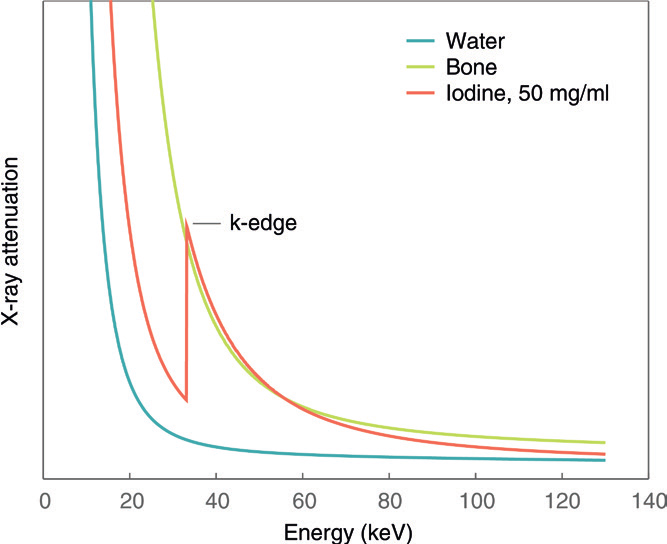
Figure 4:The linear attenuation coefficient () of bone (green), water (blue) and iodine (orange) plotted as a function of the incoming X-ray photon energy. Iodine exhibits a k-edge, characterised by a sharp increase in attenuation at a specific energy, making it unsuitable to be modelled as a linear combination of bone and water. Figure reproduced from Willemink et al., 2018
The linear attenuation coefficient (), which describes how a material attenuates X-rays, depends on both the material and the photon energy, as shown by the attenuation curves in Figure 4. For bone, water and other forms of tissue in the human body these attenuation curves can be assumed smooth within the energy range used Willemink et al., 2018. However, contrast agents such as iodine display one or more K-edges, sudden increases in attenuation at specific energies, which cannot be accurately modeled by a simple combination of water and bone. In this work, only bone and water will be used. If a contrast agent were to be involved, a 3rd material must be added to compensate for any possible k-edges.
In this work the reconstructed image of the PCD CT scan will therefore consist of 2 images. One displaying the bone density and one displaying water density. The linear attenuation coëfficient of any material within the phantom can then be described as:
where is the weight of material b, representing the amount of material b present in the voxel, and describes the attenuation coefficient of the basis material b. Combining equation (1) and (3) gives an expression for the photon count at the detector:
where represents the effictive x-ray spectrum which includes both the shape of the X-ray source spectrum and how the detector responds to photons of different energies. The detector does not detect all photon energies equally well, some energies are absorbed more efficiently than others or may be missed due to noise or other effects. is the weight of material b along line path .
Projection algorithms
To view the cross-sectional image of an object from these measurements, either from a detector or from simulations using equation (2), a reconstruction algorithm needs to be used. Filtered back projection (FBP) is an analytical reconstruction algorithm where during reconstruction each projection is spread back across the image plane along the same angle it was acquired. This often leads to blurry images as the intensity is spread along lines rather than concentrated at specific points Zeng, 2001. A filter is used to help sharpen the image and reduce blurring artifacts. FBP can be used for spectral CT scans by a two-step image based method. The first step is to reconstruct an image for each energy bin and these intermediate images are then decomposed into material-dependent images Mory et al., 2018.
The two-step, image based method has several drawbacks. First, streaking artifacts (lines across the image) often occur as the attenuation coefficient is still averaged over a line. Secondly, the first step leads to a loss of information as there is no one-to-one mapping between the projections and the images. The second step is unable to compensate for this loss as it has no access to the photon counts. Recently one-step methods have been proposed which reconstruct material-specific images directly from photon counts Mechlem et al., 2018. These are all iterative methods as no analytical inversion formula exists.
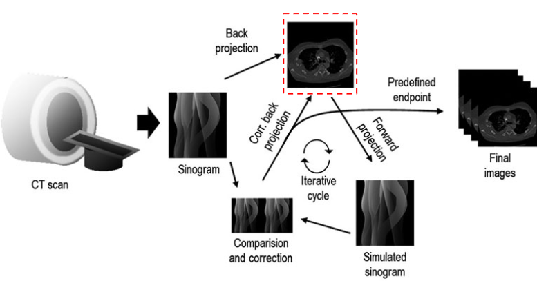
Figure 5:An overview of an iterative reconstruction algorithm. From the measured projections a reconstructed image is estimated. This image is then iteratively compared with the original sinogram in the forward projection and corrected until a predefined endpoint. Figure reproduced from Arndt et al., 2021
An iterative reconstruction algorithm starts with an initial guess of the image and, at each iteration updates the image to better match the measured data. Figure 5 shows the full cycle, from CT scan to final images. A forward projection as described by equation (2) is used to simulate a sinogram for the guessed image. The simulated sinogram is compared with the measurements according to a cost function. The cost function depends on how well the image assumption explains the measured photon counts (data fidelity term), and how smooth, or physically plausible the images is (regularization term) Zhang et al., 2018. The iterative algorithm used, uses a separable quadratic surrogates (SQS) cost function. The guess is then updated and the cycle repeats untill a predefined endpoint.
A downside to the iterative algorithm is the computational time. For each iteration there is a forward projection and a backprojection, as well as an error calculation. Also a large amount of iterations are needed to get to an accurate solution. This work will look at including machine learning to replace the iterative steps.
Machine learning - Neural networks
Neural networks are a subset of machine learning and play a crucial role in deep learning algorithms. A simple, fully connected neural network consists of nodes stacked in layers: an input layer, one or more hidden layers and an output layer.
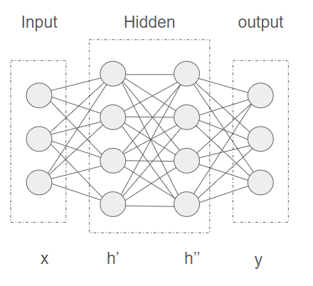
Figure 6:A neural network consisting of 3 input nodes, 2 hidden layers with 4 nodes each and an output layer with 3 nodes. The input values are represented by an array x, the hidden layers by array h’ and h’’ and the output layer by y.
All nodes in a layer are connected to an adjacent layer by weights. Figure 6 shows a simple neural network, where input layer x and first hidden layer h’ are connected by a matrix of weights , the states of the first hidden layer can be calculated as
with representing the learnable weights connecting the input neuron to the neuron in the first hidden layer, and σ is an activation function (e.g., sigmoid or softmax) that scales the output between 0 and 1 to stabilise the network and to introduce non-linearity. The bias term is another learned parameter which offsets the output. Equation (5) can be repeated for every following layer where the output of a layer is used as an input to calculate the following layer.
Neural networks are generally trained using the backpropagation algorithm, which relies on a dataset consisting of input-output pairs. During training, the network processes each input and generates an output, A cost function determines the error between the network’s output and the target output. This cost function guides the learning process by indicating how far the network’s predictions are from the desired outputs. The backpropagation algorithm will look at how each weigth in the network needs to change to minimalise the error.
Machine learning - Convolutional neural network
A convolutional neural network (CNN) can be used to more accurately extract features from images for processing, where a feature is a characteristic or pattern in the input data. A CNN consist of a kernel (also called a filter) and one or more channels. The kernel is smaller than the input data but has the same number of dimensions (e.g., 2D for 2D images). The kernel contains weights that are learned during training.
The kernel is moved across the input data, performing element-wise multiplication with the region of the input it covers, followed by a sum. This operation extract features such as edges, textures and shapes Yamashita et al., 2018. We can write the output feature map of a convolutional layer as
where are spatial indices, the image, the relevant kernel with learnable weights and the kernel indices. After a convolution layer, can be either vectorised to be used as an input for a fully connected layer as described in equation (5) or used as an input for a second convolution layer. Due to a kernel only working on adjecent pixels, convolutional layers extract local features.
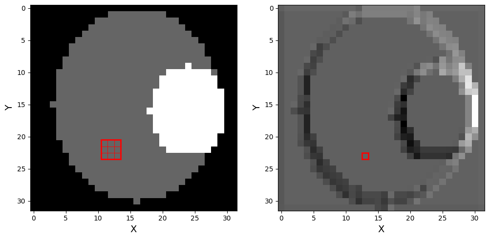
Figure 7:left : original phantom with a 2D 3x3 randomly initialised kernel drawn on top. each individual square represents a pixel, with the outer square representing the kernel. right : phantom after a 2D convolution layer with randomly initialised weights has been applied.
The left part of Figure 7 shows a 3x3 convolution kernel with randomly initialised weights (red) placed on a phantom and the right part of the figure shows the image of the phantom after the convolution. Even with randomly initialised weights, there is already an edge-detection like pattern. The image on the right is called a feature map, as each pixel represents higher-level information of the original image.
A CNN typically consists of multiple layers stacked on top of each other, allowing deeper feature extraction. Early layers can detect simple features like edges, while deeper layers can detect more complex structures like shapes and objects.
Machine learning - U-Net architecture
Multiple convolution layers can be combined to form an encoder. An encoder generates an abstract representation of an input image by repeatedly performing convolution and progressivly reducing the size of the image. This reduction is achieved using max pooling layers, which divide the input into rectangular regions and takes the maximum value from each region, reducing the image size and allowing the network to capture more abstract and higher-level data between layers.
Similarly a decoder can be used generate an output image from the abstract representation. A decoder uses deconvolution layers which progressively increases the size of the image, adding features back in at each step to refine the output.
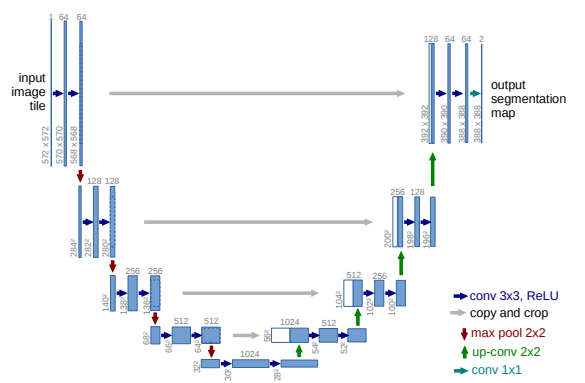
Figure 8:A U-Net architecture for an image with a 32x32 lowest possible resolution. Each blue square represents a multi-channel feature map with the amount of channels denoted on top of the box. Gray arrows represent cross over layers with the white boxes representing copied layers from the encoder Figure reproduced from Oktay et al., 2018
By combining an encoder and a decoder, a U-Net can be constructed as illustrated in Figure 8. Between each layer of the encoder and decoder part of the network, there is a skip-connection layer which copies the feature map from the encoder layer to the decoder layer. This allows the decoder to use features during reconstruction which might have been lost while encoding the image.
Machine learning - Attention gate
For feature extraction from images where both local and non-local features are of importance, convolution layers can be combined with attention mechanisms. An attention mechanism allows machine learning models to attend to the most relevant parts of the input data Vaswani et al., 2017.
An attention mechanism takes the input vector and multiplies it by an attention score to preserve only the activations relevant to the task. To calculate , an intermediate attention score (the attention score for layer l) can be defined as
where the gating feature vector, and weight matrices similar to those used in equation (5), another learned linear transformation, and learned biases similar to the bias in equation (5), and an activation function. The gating feature vector provides contextual information from higher-level layers. It acts as a control signal that guides the attention mechanism, helping it decide which parts of the input to focus on. The final attention coefficient , the final attention mask that says which parts of the feature map should be passed forward, is then calculated as
with representing the learned parameters of the attention block: all weights and biases. The final output of the attention gate is
where regions get where less important regions get . Due to the gating vector is the attention mechanism able to focus on non-local features.
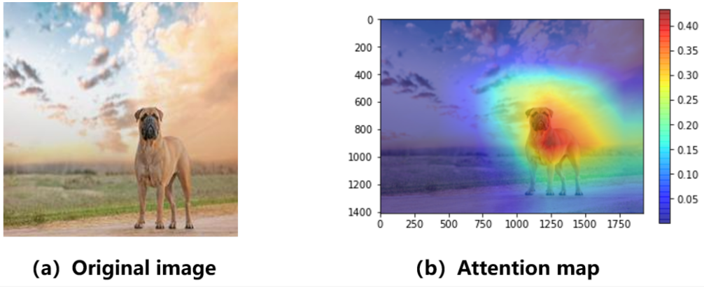
Figure 9:Example image from an attention-based network trained to label images. Image a shows a picture of a dog which the network needs to label and image b shows the attention map which is the value of per pixel. Figure reproduced from An & Joe, 2022
An example has been taken from An & Joe, 2022, where an attention-based network has been trained to label images. An input image can be seen on the left in Figure 9 where the label is supposed to be ‘dog’. A heatmap for the value of is shown on the right where we can see the attention mechanism provides a strong focus on the part of the image where the dog is located.
Machine learning - Attention U-Net
Attention mechanisms can be added to the skip-connections of the U-Net model in Figure 8, allowing the network to focus on non-local features during the reconstruction of the image. The combination of attention mechanisms and convolutional layers can be used by the attention U-Net (AttU-Net) to recognise certain features like edges and to make connection between features in different parts of the image Oktay et al., 2018.
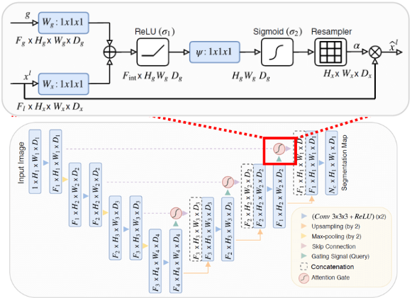
Figure 10:Schematic overview of a U-Net model with attention gates added to the skip-connections. The inset (top) shows a zoomed-in view of an attention gate, the gating signal is taken from the previous decoding layer and the input is the skip-connection layer. Figure reproduced from Oktay et al., 2018
The attention mechanism uses the gating signal to modulate the features passed through the skip connection, which allows the network to selectively emphasize relevant spatial features and suppress irrelevant or noisy information. Each skip connection uses the output of the previous decoder layer as a gating signal to control which encoder features are passed forward, as illustrated in Figure 10.
Method
Overview
A machine learning model will be trained to use information from sinogram space to adjust images in image space. The network will be trained to perform this conversion in iterative steps similar to the iterative reconstruction method described in Mechlem et al., 2018.
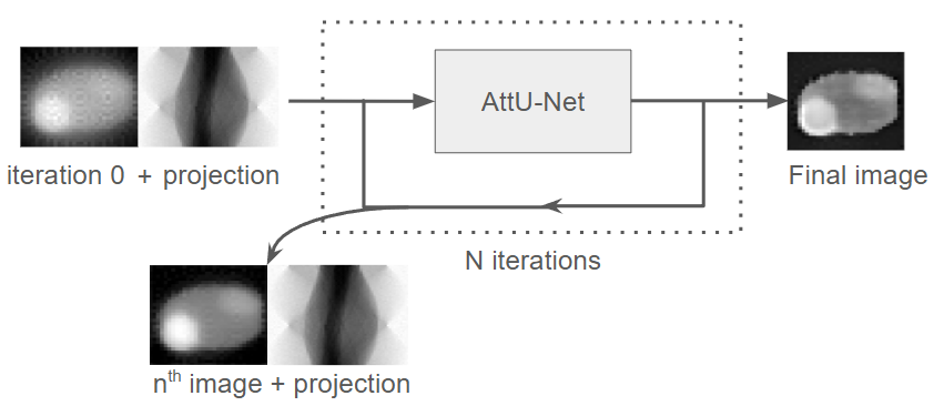
Figure 11:Schematic overview of the model workflow. The input to the model consists of the first reconstructed image from the iterative algorithm (called iteration 0 for the AttU-Net model) combined with the corresponding projection (sinogram) data. The network processes this input iteratively, where the output of the iteration is used as the input for the iteration, while the projection data remains constant. After N iterations, the final reconstructed image is produced.
An overview of the model workflow is shown in Figure 11. The network is designed to use the first reconstructed image from the iterative algorithm (called iteration 0 for the AttU-Net model) combined with the projection matrix and refine the reconstructed image across 20 iterations. The output image of an iteration is used as an input for the following iteration, making sure the projection matrix remains constant. After 20 iterations, the output of the network is used as the final image.
Generating phantoms
The training data consists of phantoms generated according to a set of rules for which projections are simulated. These projections are used by the iterative algorithm, where the intermediate images, as illustrated by the red, dotted line in Figure 5, are used as training data for the model. The phantoms are randomly generated according to a set of rules:
each phantom is 32x32x32 pixels and consists of 2 channels, one for bone and one for water.
each phantom has a main, elliptical body centered in the image consisting of a low mass density of both water and bone (both densities uniformly distributed between 0.1 and 0.6).
The center of the body can be randomly offset by −3 to +3 pixels in both the x and y directions (uniform distribution).
The size of the main body varies, with the distance between the points on the axis varying between 1 and 3 pixels uniformly distributed.
Each phantom has 2 internal features, represented as smaller elliptical regions within the main body.
Each feature has either a higher bone density or a higher water density than the other.
The bone and/or water density cannot be lower in a feature than the main body
Each feature represents a distinct elliptical region. Because photon counting detectors (PCDs) allow differentiating tissue types, we assign one feature a higher bone density and the other a higher water density. This design ensures that the network is trained on a task relevant to the clinical use of PCDs. These rules have been implemented in python to generate a sample of phantoms as seen in the supporting notebooks.
Acquiring data
For 506 phantoms, detector measurements are simulated. These measurements are acquired with 32 angles per phantom. Next, each set of detector measurements are reconstructed using the iterative algorithm, the predefined endpoint as shown in Figure 5 is defined as 40 iterations. These iterations, illustrated by the red, dotted line in the same figure, are used to construct input-output pairs for training the model. Using a stride (how many iterations to skip between input and output images), the input is defined as the image from the iteration, with a corresponding output image taken from the iteration.
Using a stride between input and output images allows the model to learn from a wider variety of scenarios within the same training time. In this work, a stride of 4 is used. This work made use of 506 phantoms, which generated 4554 input-output pairs.
Attention based U-Net
To enable the network to learn how features in the image space and the projection (sinogram) space attend to eachother, a U-Net architecture with attention mechanisms integrated into the skip connections is used (AttU-Net) as described by Oktay et al., 2018. The attention gates help the model to focus on which parts of the sinogram contribute to specific image regions.
The AttU-Net model is illustrated in Figure 10. The architecture consists of five convolutional encoder blocks, a bottleneck block, and five decoder blocks. The number of channels increases through the encoder (64, 128, 256, 512 and 1024), and then decreases symmetrically through the decoder. The output layer applies a sigmoid activation to produce voxel-wise probabilities. The model has been implemented in Python using Pytorch in the supporting notebooks
The model is trained on an NVDIA Tesla A100, with 4 hours allocated per run. In total 6 runs were completed, which resulted in 180 epochs (20 epochs per run). The model uses MSELoss as a loss function and Adam optimisation, which is a stochastic gradient descent method. The learning rate is set to 0.001, which is commonly used with Adam optimisation Kingma & Ba, 2014. An implementation of the training function can be seen in the supporting notebooks
Shaping the data
The AttU-Net model takes an image as input and produces an image of the same size as an output. Since 2 different images are used (the image and the projection), these must be combined into a single matrix. The projection matrix has dimensions (number of projections) x (z pixels detector) x (y pixels detector), where this work uses 32 projections and a detector of 64 by 44 pixels as set for the simulations in the supporting notebooks.
Aditionally, due to the pooling layers all dimensions must be powers of 16 as to not get an uneven amount of devisions. The projection matrix is originally 32 x 44 x 64 pixels, which we can pad with zeros to 32 x 48 x 64 pixels. The image will is 32 x 32 x 32 pixels which we can pad to 32 x 48 x 32 to fit the dimensions of the projections. The final input set to the network will be 10 x 32 x 48 x 96 as we use 10 channels in total. The output will be 2 x 32 x 48 x 96, 2 output channels corresponding the bone and water images.
Validation
20 phantoms are used as a validation set, generated under the same conditions and rules as those used for training. The performance of both the AttU-Net model and the iterative algorithm will be compared by calculating the root-mean-square (RMS) error between a reconstructed image and the ground truth (GT) image. The RMS error is calculated as
where and are the pixel values at position in image 1 and image 2, respectively. N is the total number of pixels in the image, 32768 pixels in this case.
results
Visualisation reconstruction
During evaluation the model has been run on 20 validation sets generated under the same conditions and rules as those used for training. By taking the first image from the iterative algorithm, 20 reconstructions can be made using the proposed AttU-Net model.
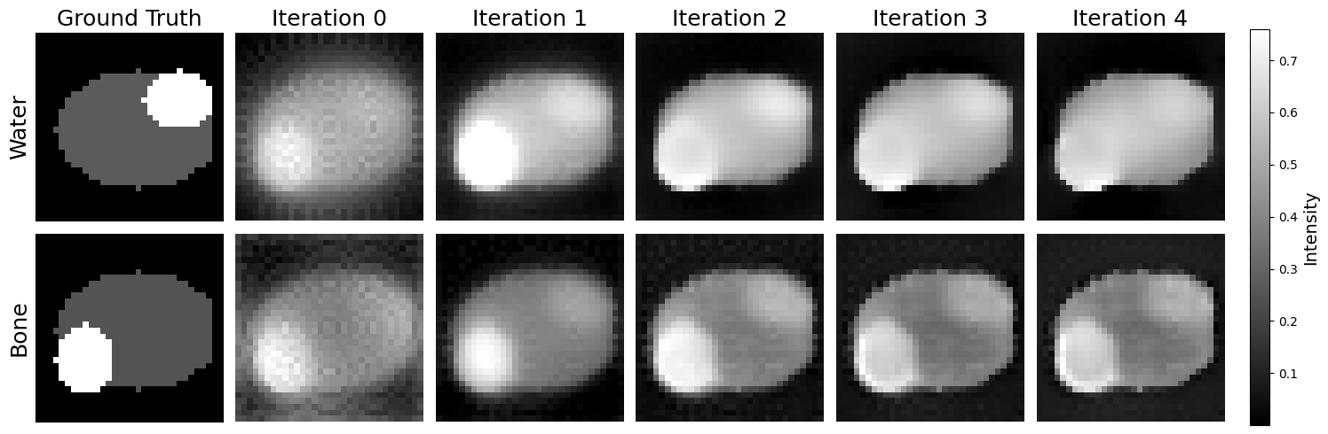
Figure 12:Top row (water), left to right: Ground truth (GT) water image; iteration 0 (first reconstruction) from iterative algorithm; subsequent reconstructions by the model. Bottom row (bone), left to right: GT bone image; iteration 0 (first reconstruction) from iterative algorithm; subsequent reconstructions by the model.
The first 4 reconstructions of the second phantom are displayed in Figure 12 and the first column displays the ground truth (GT) images as a reference. The rows show the reconstruction process using the model for water and bone respectively, where each column is an iteration. In the GT images, distinct features are visible: a bone structure in the lower left quadrant and a water structure in the top right quadrant. These serve as reference to evaluate the reconstruction quality.
The first reconstruction shows that the AttU-net model accurately recongnises the key features of the phantom, however the water feature is faint in the water density image. As reconstruction progresses, the overall water density increases while the edges between distinct features of the phantom are blurred. The bone density image looks to converge to a state where the phantom’s body has a lower density, with both water and bone features present.
Visualisation comparison
To better understand the quality of the images compared to the iterative algorithm, the iterative algorithm has been used to reconstruct the phantoms as well using the same parameters as used during training.
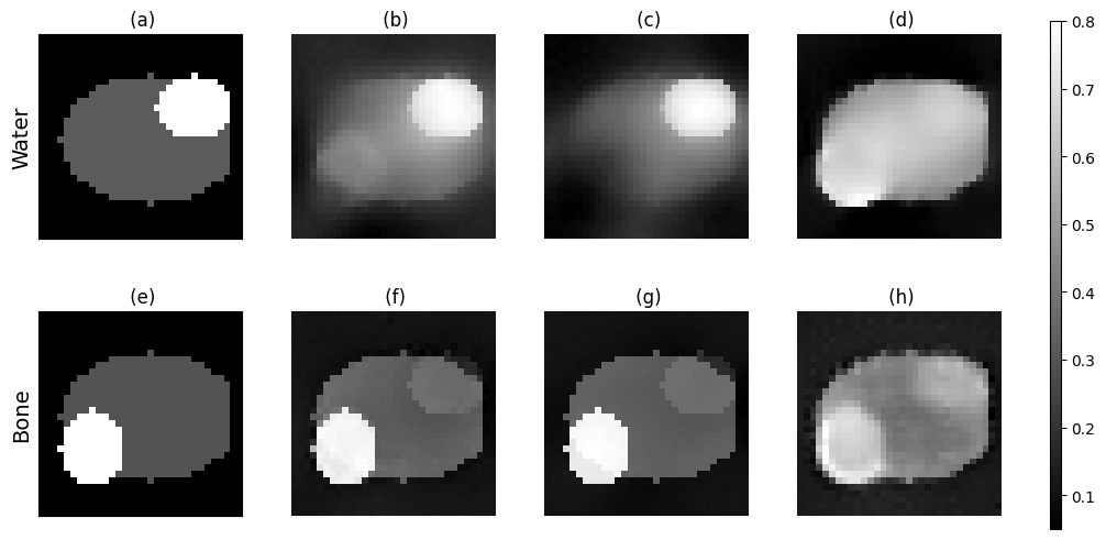
Figure 13:(a) GT water image (b) smallest RMS water image iterative algorithm (c) water image from last iteration iterative algorithm (d) water image reconstructed by the model after 3 iterations (e) GT bone image (f) smallest RMS bone image iterative algorithm (g) bone image from last iteration iterative algorithm (h) bone image recontructed by the model after 3 iterations.
Looking at the reconstructions corresponding to the smallest root mean square (RMS) error across all iterations (panel b and f), both water and bone features are present in their respective images. However the iterative algorithm does not fully distinguish between the materials of the two features, as the water feature can be faintly seen in the bone images and vice versa. For the final iteration of the iterative algorithm (panel c and g), the water image shows a clear reduction of the bone feature. This indicates an overcompensation compared to panel b.
Eventough more blurry, the bone image reconstructed by the AttU-Net model has the same level of pattern recognition as the iterative algorithm. The model was unable to recognise these features in the image for water, while the iterative algorithm does. The images generated by the model also have a lower contrast between features compared to the iterative approach.
RMS over time
By calculating the RMS error at each iteration for both the iterative algorithm and the model with the ground truth (GT) image, we can compare the reconstruction errors as a function of time.
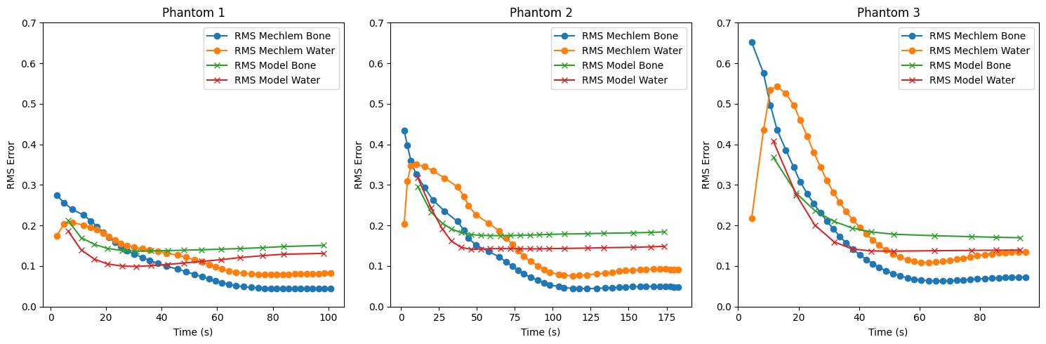
Figure 14:RMS error over time for three phantoms reconstructed using both the iterative method (orange: water; blue: bone) and the proposed AttU-Net model (red: water; green: bone).
Figure 14 shows the RMS error over time for bone and water images reconstructed by both methods for the first 3 phantoms from the validation set, where the second phantom can be seen in Figure 12 and Figure 13. The AttU-Net model has been run for as long as it took for the iterative algorithm to complete all 40 iterations. In all three cases, the model achieves a lower initial error but converges to a larger error compared to the iterative algorithm. For both algorithms the RMS error of the water images converges to a higher value than the RMS of the bone images.
Table 1:The average time (in seconds) required for each method to reach a specified error threshold , calculated for 20 sets.
| Iterative | 4.75 | 7.38 | 13.58 | 23.68 | 42.03 |
| AttU-Net | 9.35 | 10.48 | 14.09 | 23.00 | - |
Looking at a dataset of 20 phantoms, the average time taken for the first iteration of the model is 9.3 seconds. Table 1 shows the average time taken for each model to reach a specific RMS error threshold . The time for the AttU-Net model to reach is equal to the average time taken to complete one iteration. The AttU-Net model failed to produce an output image with a RMS error lower than 0.1.
The average values shown in Table 1 are highly influenced by the fluctuating range of error values produced by both methods. As seen in Figure 14, the maximum error across methods for phantom 1 is 0.29 while this is 0.66 for phantom 3. To provide a more meaningful comparison between methods, we define an average speedup as the ratio between the time the iterative approach takes to reach the same RMS error that the AttU-Net model achieves after one iteration, and the time taken for that one AttU-Net iteration. Based on this definition:
The average speedup for bone for the first iteration is 1.44x, meaning the iterative method takes 44% more time to reach the same error
The average speedup for water is 1.17x, or 17% more time.
On average, the speedup for the first iteration is therefore 30%. Beyond this initial comparison point, calculating further speedups becomes less meaningful, as the RMS error of the model remains too high to yield visually useful results.
Further visual analysis
Inpsecting all reconstructed images of the 20 phantoms as done in the supporting notebook, it can be noted some reconstructions performed by the iterative algorithm are visually far from the GT.
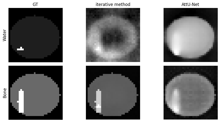
Figure 15:The GT images of phantom 17 from the validation set, with the final iterations of the iterative method and the AttU-Net model for both water and bone.
One such case is displayed in figure Figure 15 where phantom 17 can be seen, reconstructed using both the iterative algorithm and the AttU-Net model. The GT has both the water and the bone features located in the lower-left quadrant. For the water density image reconstructed using the iterative approach it can be seen there are no recognisable features from the GT present, however there does seem to be a significant lack of water in the center of the image.
The AttU-Net model has, similarly to phantom 2, a relatively constant value throughout the phantom for the water image, while the bone reconstruction does accurately show the bone feature.
Attention map
An attention map similar to Figure 9 can be generated for the first skip connection of the AttU-Net model.
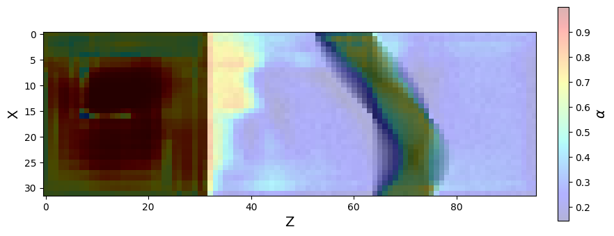
Figure 16:An attention map illustrating the regions of the input data that the attention mechanism in the first skip connection of the AttU-Net focuses on. The image was generated by running the model on a phantom and extracting the values of the attention coefficients . A 2D slice (at ) was taken from the 3D attention volume.
Figure 16 shows an attention map from the trained AttU-Net model. The map visualizes the attention coefficients for the first skip connection. In this specific case, the attention gate focuses on the lower-intensity regions of the sinogram, which are known to contain the most informative features for reconstructing the imaged object.
Discussion
Model is only as good as the data
The trained AttU-Net model reconstructed 20 images using a validation set of phantoms. The first four reconstructions of the second phantom are shown in Figure 12 where the model successfully identifies features present in the phantom but fails to clearly distinguish between bone and water.
Looking at the RMS error over time for the first three phantoms as plotted in Figure 13, reveals that the AttU-Net model initially achieves a lower RMS error compared to the iterative algorithm but eventually converges to a higher value.
When analyzing the final iterations of the iterative algorithm across all 20 validation phantoms, it can be seem some images do not converge to a visually accurate state as displayed in Figure 15. Since the AttU-Net model was trained on these results, including those that failed to converge, this likely explains why the model itself also fails to converge effectively in later iterations. For future work, it is recommended to set an RMS error threshold and use only iterative reconstructions that meet this criterion for training.
non-machine learning speedup
Looking at the software implementation for each method, the AttU-Net is more optimised than the iterative algorithm. The AttU-Net makes use of the PyTorch framework which is highly optimised for machine learning tasks. The iterative algorithm has been implemented from scratch and does not include any form of optimisations, which leads to an unfair comparison between the two algorithms.
One way of optimising the iterative algorithm is parallelizing the computation of the SQS cost function. The SQS cost function is designed to look at the error relative to only it’s neighbour, so it is part of the code most easily parallelised.
Image size, model size, number of projections
The model currently reconstructs images of size 32 × 32 × 32 pixels, which is too small for clinical applications. Future work should explore how performance and reconstruction time scale with increasing image size. Key factors to consider include:
Number of projections: Larger images require more projections to fully capture all relevant information.
Detector size: As image size increases, detector dimensions must also increase.
Network size: To accommodate the added complexity of larger images, the network architecture must scale too.
Hardware requirements: The current model already occupies 0.5 GB. Scaling up the network will demand additional storage and more powerful hardware.
To properly compare running times, it is recommended to develop an AttU-Net-style model capable of reconstructing larger images to the same RMS error within a fixed number of iterations. This ensures that performance comparisons do not come at the cost of reduced reconstruction accuracy.
Adding cross attention between spaces
Cross attention can implemented between two images as done by Alaluf et al., 2023, where features from one image are used as a gating signal for an attention mechanism that processes the other image. Currently, two different spaces, image space and projection space, are added together in the same matrix. By using cross-attention, these spaces can be treated separately, with the attention mechanism serving as the interface between them. This allows for a more structured and interpretable flow of information between domains.
Regularisation term
Since the AttU-Net is used to reconstruct CT scan images, its outputs must be clinically meaningful and physically plausible. To help guide the model toward producing more realistic reconstructions, a regularisation term can be introduced during training and reconstruction Ge et al., 2023. This term can incorporate physical constraints into the learning process, encouraging the model to generate outputs that not only appear correct but also align with the physical reality of CT imaging.
For example, by penalising discrepancies between the forward projections of the reconstructed image and the actual measured sinogram data, the model is discouraged from producing outputs that deviate from what is physically observable. This helps the network learn to reconstruct features that are consistent with the measurement process, reducing the risk of hallucinated structures or anatomically implausible results.
Conclusion
The proposed Attention U-Net (AttU-Net) model successfully recognises the outline of bone and water features within phantom images during density reconstruction. However, it fails to reliably distinguish between the two materials. This limitation is particularly relevant, as the ability to separate different materials, such as bone and water, is a key reason to use photon-counting detectors (PCDs) in imaging.
Despite this, the model demonstrates significant promise. It achieves, in a single forward pass, the same reconstruction error that requires multiple iterations of a traditional algorithm; resulting in a 30% reduction in time to reach an equivalent RMS error. This highlights the model’s potential to accelerate, or even replace, conventional iterative techniques. While the model reaches this level quickly, it converges to a higher final RMS error than the iterative method it is tested against.
To move towards deploying the model in clinical settings, the model must be scaled to accommodate higher-resolution images. This will require increasing the network’s capacity, such as increasing the amount of layers or increasing the amount of channels, to preserve details. Additionally, training data should be filtered by applying a threshold to the RMS error of the final iterative reconstructions, ensuring only high-quality examples are used for training.
- Pietzsch, J. (2025). Perspectives: With a little help from my friends. https://www.nobelprize.org/prizes/medicine/1979/perspectives/
- Taguchi, K., & Iwanczyk, J. S. (2013). Vision 20/20: Single photon counting x-ray detectors in medical imaging. Medical Physics, 40(10), 100901. 10.1118/1.4820371
- Mechlem, K., Ehn, S., Sellerer, T., Braig, E., Münzel, D., Pfeiffer, F., & Noël, P. B. (2018). Joint Statistical Iterative Material Image Reconstruction for Spectral Computed Tomography Using a Semi-Empirical Forward Model. IEEE Transactions on Medical Imaging, 37(1), 68–80. 10.1109/TMI.2017.2726687
- Oktay, O., Schlemper, J., Le Folgoc, L., Lee, M., Heinrich, M., Misawa, K., Mori, K., McDonagh, S., Hammerla, N. Y., Kainz, B., Glocker, B., & Rueckert, D. (2018). Attention U-Net: Learning Where to Look for the Pancreas. arXiv Preprint arXiv:1804.03999. 10.48550/arXiv.1804.03999
- Vaswani, A., Shazeer, N., Parmar, N., Uszkoreit, J., Jones, L., Gomez, A. N., Kaiser, L., & Polosukhin, I. (2017). Attention Is All You Need. arXiv Preprint arXiv:1706.03762. 10.48550/arXiv.1706.03762
- Kamalian, S., Lev, M. H., & Gupta, R. (2016). Computed Tomography Imaging and Angiography – Principles. In M. J. Aminoff & R. B. Daroff (Eds.), Handbook of Clinical Neurology (Vol. 135, pp. 3–20). Elsevier. 10.1016/B978-0-12-802973-2.00001-7
- Leuschner, J., Schmidt, M., Baguer, D. O., & Maass, P. (2019). The LoDoPaB-CT Dataset: A Benchmark Dataset for Low-Dose CT Reconstruction Methods. arXiv Preprint arXiv:1910.01113. 10.48550/arXiv.1910.01113
- Venkatesh, E., & Elluru, S. V. (2017). Cone beam computed tomography: basics and applications in dentistry. Journal of Istanbul University Faculty of Dentistry, 51(3 Suppl 1), S102–S121. 10.17096/jiufd.00289
- Yang, F., Zhang, D., Huang, K., & Shi, W. (2017, February). Projection Matrix Acquisition for Cone‑Beam Computed Tomography Iterative Reconstruction. Proceedings of SPIE – The International Society for Optical Engineering. 10.1117/12.2269014
- Marth, A. A., Marcus, R. P., Feuerriegel, G. C., Nanz, D., & Sutter, R. (2023). Photon-Counting Detector CT Versus Energy-Integrating Detector CT of the Lumbar Spine: Comparison of Radiation Dose and Image Quality. AJR. American Journal of Roentgenology, 222(1). 10.2214/AJR.23.29950
- Antsiferov, P. S. (2003). The Characteristic X-Ray Spectra of Free Atoms of Metals. Central European Journal of Physics, 2(2), 268–288.
- Taguchi, K., Ballabriga, R., Campbell, M., & Darambara, D. G. (2022). Photon Counting Detector Computed Tomography. IEEE Transactions on Radiation and Plasma Medical Sciences, 6(1), 1–4. 10.1109/TRPMS.2021.3133808
- Willemink, M. J., Persson, M., Pourmorteza, A., Do, T., & Fleischmann, D. (2018). Photon-counting CT: Technical Principles and Clinical Prospects. Radiology, 289(2), 293–312. 10.1148/radiol.2018172656
- Zeng, G. L. (2001). Image reconstruction—a tutorial. Computerized Medical Imaging and Graphics, 25(2), 97–103.
- Mory, C., Sixou, B., Si-Mohamed, S., Boussel, L., & Rit, S. (2018). Comparison of five one-step reconstruction algorithms for spectral CT. Physics in Medicine and Biology, 63(23). 10.1088/1361-6560/aaeaf2