In this task we will discuss the performances of both models, the types of errors made and recommendations for future development. Throughout the task, I will refer to the model combining HOG and GLCM feature extraction with a RF classifier designed in task 1 as model 1. I will refer to the pre-trained ResNet18 model with a Random Forest classifier as model 2.
Source
import pandas as pd
import numpy as np
import matplotlib.pyplot as plt

# load df from my_dataframe.csv
train_df = pd.read_csv('train_dataframe.csv', index_col=0)
val_df = pd.read_csv('val_dataframe.csv', index_col=0)

# load this: report_df.to_csv('task1_classification_report.csv', index=True)
report_1_df = pd.read_csv('task1_classification_report.csv', index_col=0)
report_2_df = pd.read_csv('task2_classification_report.csv', index_col=0)

# round both reports to integer
report_1_df = report_1_df.round(2)
report_2_df = report_2_df.round(2)

misclassified_images_1 = pd.read_csv('misclassified_images_1.csv')
misclassified_images_2 = pd.read_csv('misclassified_images_2.csv')
Comparative Analysis
Model 2, which combines the pre-trained ResNet18 with a Random Forest classifier, performs significantly better at recognizing all defects than Model 1, which uses HOG and GLCM feature extraction with a Random Forest classifier. The average precision of Model 2 is 0.99, compared to 0.90 for Model 1.
One reason is the types of features extracted by the ResNet18 model. The model consists of multiple convolutional layers, which allows the extraction of hierarchical and multi-scale features such as fine textures, local shapes, and repeated patterns. The model designed in task 1, on the other hand, makes use of only two distinct feature types, HOG and GLCM, which primarily capture edges, gradients, and simple textural statistics, limiting the ability of the classifier to distinguish more subtle or complex defects.
The ResNet18 model has been trained on a large dataset, (ImageNet), which contains over 1.2 million images across 1,000 classes. This exposure allows the model to learn a wide variety of visual patterns, from simple edges to complex textures and object structures. As a result, even when applied to grayscale steel surface images, the model can extract rich and generalizable features that help the Random Forest classifier distinguish between different types of defects more effectively than handcrafted features alone.
I would also like to note that the RF classifier in task 1 is trained using 18,512 input features, while the RF classifier in task 2 is trained using only 512 input features. The fact that model 2 achieves higher precision demonstrates how curated and informative the ResNet-derived features are, with the ResNet part of the model effectively performing high-level preprocessing before classification.
Source
# import Image from PIL
from PIL import Image

# for each misclassified image, plot the image, the true label and the predicted label which is type and predicted_type
for i, row in misclassified_images_1.iterrows():
    img = Image.open(row["filepath"]).convert("RGB")
    plt.subplot(1, len(misclassified_images_2), i + 1)
    plt.imshow(img)
    plt.title(f"True: {row['type']}\nPred: {row['predicted_type']}")
    plt.axis('off')
plt.show()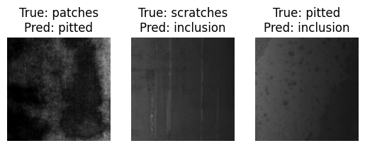
which all depict different ‘problems’ regarding the model.
Patches which are classified as a pitted-surface. This mistake can be due to the stepsize used to collect the GLCM features, where the largest stepsize of 8 might not provide enough distance to properly contextualise the defect.
Scratches classified as inclusions. This is a classification error also hard to spot by eye. We will see model 2 equally struggle with this. This is most likely due to both defects consisting of straight, high contrast lines.
A pitted-surface clasified as an inclusion. This misclassification can reasonably be due to the low image quality, with a general gradient between the upper left corner and lower right corner. The HOG feature might have picked up a gradient line, which can easily be classified as an inclusion.
Model 2
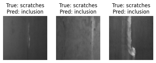
For the model from task 2, there are only 3 mistakes in classification. For each image, a scratch is classified as an inclusion.
Source
# for each misclassified image, plot the image, the true label and the predicted label which is type and predicted_type
for i, row in misclassified_images_2.iterrows():
    img = Image.open(row["filepath"]).convert("RGB")
    plt.subplot(1, len(misclassified_images_2), i + 1)
    plt.imshow(img)
    plt.title(f"True: {row['type']}\nPred: {row['predicted_type']}")
    plt.axis('off')
plt.show()
To visualise the difference between images showing scratches and images showing inclusions, we can display 10 images from the dataset
Source
import matplotlib.pyplot as plt
from PIL import Image

# Get 10 inclusions and 10 scratches from val_df
inclusion_images = val_df[val_df["type"] == "inclusion"].head(10)
scratch_images = val_df[val_df["type"] == "scratches"].head(10)

all_images = [inclusion_images, scratch_images]
all_labels = ["Inclusion", "Scratches"]

# Create figure (from matplotlib documentation)
fig, axs = plt.subplots(2, 10, figsize=(20, 4))

for row_idx, (images, label) in enumerate(zip(all_images, all_labels)):
    for col_idx, filepath in enumerate(images["filepath"]):
        img = Image.open(filepath)
        axs[row_idx, col_idx].imshow(img, cmap='gray')
        # Hide ticks but keep label
        axs[row_idx, col_idx].set_xticks([])
        axs[row_idx, col_idx].set_yticks([])

    # Set vertical row label on leftmost subplot
    axs[row_idx, 0].set_ylabel(label, fontsize=14, rotation=90, labelpad=15, va='center')

plt.tight_layout()
plt.show()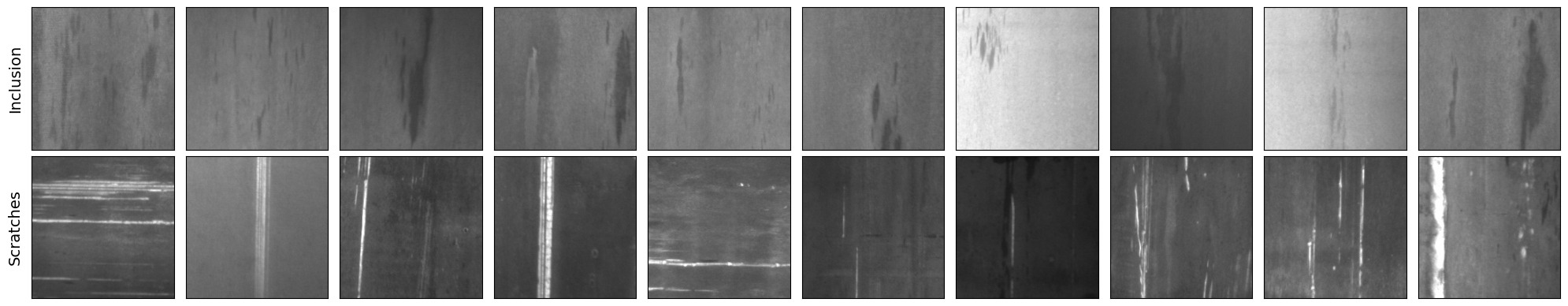
Again, both defects can be recognised by long streaks in a relatively straight line. It is highly likely the ResNet model, which consists of multiple convolution layers, recognises some of these features as similar.
One interesting thing to note, is how in this subset of the data, inclusions seem to have a darker colour than the surroundings, while scratches appear lighter. This can be used for a further experiment to try and distinguish the 2 types of defects.
To summarise: Model 2, with its more comprehensive feature representation, is better able to classify defects. Both models, however, still have difficulty distinguishing between scratches and inclusions.
Future Strategy & Next Steps
Future Strategy
The first experiment I would recommend with GPU access, is to append a new classification layer to the ResNet18 model which we can train using our own data. By training the model to our own dataset, the features will be more curated to the type of images we provide. This is a tried and tested method (as done here).
Next, I would add a seventh class to the dataset consisting of images without any defects. The current model can classify the type of defect, but ideally, a camera should be able to automatically detect whether a defect is present and then classify its type. If we do not have direct access to the camera, as in this scenario, we can use parts of the surfaces adjacent to scratches, and the subimages can be cropped or resized to the correct dimensions for the model.
Finally, using the PyTorch library we can easily choose from a range of models to use for this application. One of which is the ResNet50 model, which has a deeper architecture than ResNet18, allowing it to extract more complex features. alternatively, we could use a different model which might be trained on images similar to the images in our dataset.
It’s important to note that it would be best to increase the amount of training and validation data to see how the model would perform over a broader range of images.
Data Augmentation
As mentioned in the error analysis for Model 1, some images may be misclassified due to poor image quality. One way to fix this could be to manually apply small gradients or intensity variations to the images to generate new data with similar properties.
When looking at the 10 samples of inclusion defects, all inclusions are oriented in a vertical direction. It could be interesting to explore wether this is true for the entire dataset, and if so we can generate additional training data by rotating these images.
Depending on the broader context of how the model will be used in production, we can also look at self-supervised learning. This paper refers to the same dataset and shows that defects can be detected effectively using unlabeled data, reducing the need for manual annotation.