We will load a pretrained CNN (resnet18) and remove the final classification layer. This allows us to extract a feature map consisting of 512 values.
Load data and model
First, we load the training and validation dataframes as constructed in task 1:
Source
import pandas as pd
import numpy as np

# load df from my_dataframe.csv
train_df = pd.read_csv('train_dataframe.csv', index_col=0)
val_df = pd.read_csv('val_dataframe.csv', index_col=0)

print("Head of training data loaded from file: \n",train_df.head())
Head of training data loaded from file:
filepath type id \
419 ../NEU-DET/train/images\inclusion\inclusion_44... inclusion 44
675 ../NEU-DET/train/images\patches\patches_59.jpg patches 59
748 ../NEU-DET/train/images\pitted_surface\pitted_... pitted 124
226 ../NEU-DET/train/images\crazing\crazing_87.jpg crazing 87
1163 ../NEU-DET/train/images\rolled-in_scale\rolled... rolled-in 66
hog_features \
419 [0.2369237 0.15415997 0.21013955 ... 0.213794...
675 [0.29324098 0.03451908 0.13982935 ... 0.068845...
748 [0.25374744 0.25374744 0.25374744 ... 0.115656...
226 [0.22393232 0.08401035 0.22393232 ... 0.095062...
1163 [0.19847726 0.07978102 0.13506998 ... 0.099056...
glcm_features
419 [1.27806533e+01 1.72544128e+01 8.23502513e+00 ...
675 [3.07574196e+02 4.26079543e+02 2.77419171e+02 ...
748 [2.01314322e+01 2.89945708e+01 1.39089196e+01 ...
226 [2.07342714e+02 2.65698795e+02 1.70630201e+02 ...
1163 [6.80495729e+01 1.12832959e+02 1.05307261e+02 ...
Next, we import the ResNet18 model. ResNet18 offers a strong trade-off between depth and efficiency, making it more effective than shallow models and less computationally demanding than very deep architectures like ResNet50. If necessary, we can also upgrade to ResNet50 once GPU access is approved ;)
Source
import torchvision.models as models
from torchvision.models import ResNet18_Weights

# Load a pre-trained ResNet18 model
model = models.resnet18(weights=ResNet18_Weights.DEFAULT) # parameter 'pretrained' is deprecated
print("model loaded correctly: \n", model)
Output
model loaded correctly:
 ResNet(
  (conv1): Conv2d(3, 64, kernel_size=(7, 7), stride=(2, 2), padding=(3, 3), bias=False)
  (bn1): BatchNorm2d(64, eps=1e-05, momentum=0.1, affine=True, track_running_stats=True)
  (relu): ReLU(inplace=True)
  (maxpool): MaxPool2d(kernel_size=3, stride=2, padding=1, dilation=1, ceil_mode=False)
  (layer1): Sequential(
    (0): BasicBlock(
      (conv1): Conv2d(64, 64, kernel_size=(3, 3), stride=(1, 1), padding=(1, 1), bias=False)
      (bn1): BatchNorm2d(64, eps=1e-05, momentum=0.1, affine=True, track_running_stats=True)
      (relu): ReLU(inplace=True)
      (conv2): Conv2d(64, 64, kernel_size=(3, 3), stride=(1, 1), padding=(1, 1), bias=False)
      (bn2): BatchNorm2d(64, eps=1e-05, momentum=0.1, affine=True, track_running_stats=True)
    )
    (1): BasicBlock(
      (conv1): Conv2d(64, 64, kernel_size=(3, 3), stride=(1, 1), padding=(1, 1), bias=False)
      (bn1): BatchNorm2d(64, eps=1e-05, momentum=0.1, affine=True, track_running_stats=True)
      (relu): ReLU(inplace=True)
      (conv2): Conv2d(64, 64, kernel_size=(3, 3), stride=(1, 1), padding=(1, 1), bias=False)
      (bn2): BatchNorm2d(64, eps=1e-05, momentum=0.1, affine=True, track_running_stats=True)
    )
  )
  (layer2): Sequential(
    (0): BasicBlock(
      (conv1): Conv2d(64, 128, kernel_size=(3, 3), stride=(2, 2), padding=(1, 1), bias=False)
      (bn1): BatchNorm2d(128, eps=1e-05, momentum=0.1, affine=True, track_running_stats=True)
      (relu): ReLU(inplace=True)
      (conv2): Conv2d(128, 128, kernel_size=(3, 3), stride=(1, 1), padding=(1, 1), bias=False)
      (bn2): BatchNorm2d(128, eps=1e-05, momentum=0.1, affine=True, track_running_stats=True)
      (downsample): Sequential(
        (0): Conv2d(64, 128, kernel_size=(1, 1), stride=(2, 2), bias=False)
        (1): BatchNorm2d(128, eps=1e-05, momentum=0.1, affine=True, track_running_stats=True)
      )
    )
    (1): BasicBlock(
      (conv1): Conv2d(128, 128, kernel_size=(3, 3), stride=(1, 1), padding=(1, 1), bias=False)
      (bn1): BatchNorm2d(128, eps=1e-05, momentum=0.1, affine=True, track_running_stats=True)
      (relu): ReLU(inplace=True)
      (conv2): Conv2d(128, 128, kernel_size=(3, 3), stride=(1, 1), padding=(1, 1), bias=False)
      (bn2): BatchNorm2d(128, eps=1e-05, momentum=0.1, affine=True, track_running_stats=True)
    )
  )
  (layer3): Sequential(
    (0): BasicBlock(
      (conv1): Conv2d(128, 256, kernel_size=(3, 3), stride=(2, 2), padding=(1, 1), bias=False)
      (bn1): BatchNorm2d(256, eps=1e-05, momentum=0.1, affine=True, track_running_stats=True)
      (relu): ReLU(inplace=True)
      (conv2): Conv2d(256, 256, kernel_size=(3, 3), stride=(1, 1), padding=(1, 1), bias=False)
      (bn2): BatchNorm2d(256, eps=1e-05, momentum=0.1, affine=True, track_running_stats=True)
      (downsample): Sequential(
        (0): Conv2d(128, 256, kernel_size=(1, 1), stride=(2, 2), bias=False)
        (1): BatchNorm2d(256, eps=1e-05, momentum=0.1, affine=True, track_running_stats=True)
      )
    )
    (1): BasicBlock(
      (conv1): Conv2d(256, 256, kernel_size=(3, 3), stride=(1, 1), padding=(1, 1), bias=False)
      (bn1): BatchNorm2d(256, eps=1e-05, momentum=0.1, affine=True, track_running_stats=True)
      (relu): ReLU(inplace=True)
      (conv2): Conv2d(256, 256, kernel_size=(3, 3), stride=(1, 1), padding=(1, 1), bias=False)
      (bn2): BatchNorm2d(256, eps=1e-05, momentum=0.1, affine=True, track_running_stats=True)
    )
  )
  (layer4): Sequential(
    (0): BasicBlock(
      (conv1): Conv2d(256, 512, kernel_size=(3, 3), stride=(2, 2), padding=(1, 1), bias=False)
      (bn1): BatchNorm2d(512, eps=1e-05, momentum=0.1, affine=True, track_running_stats=True)
      (relu): ReLU(inplace=True)
      (conv2): Conv2d(512, 512, kernel_size=(3, 3), stride=(1, 1), padding=(1, 1), bias=False)
      (bn2): BatchNorm2d(512, eps=1e-05, momentum=0.1, affine=True, track_running_stats=True)
      (downsample): Sequential(
        (0): Conv2d(256, 512, kernel_size=(1, 1), stride=(2, 2), bias=False)
        (1): BatchNorm2d(512, eps=1e-05, momentum=0.1, affine=True, track_running_stats=True)
      )
    )
    (1): BasicBlock(
      (conv1): Conv2d(512, 512, kernel_size=(3, 3), stride=(1, 1), padding=(1, 1), bias=False)
      (bn1): BatchNorm2d(512, eps=1e-05, momentum=0.1, affine=True, track_running_stats=True)
      (relu): ReLU(inplace=True)
      (conv2): Conv2d(512, 512, kernel_size=(3, 3), stride=(1, 1), padding=(1, 1), bias=False)
      (bn2): BatchNorm2d(512, eps=1e-05, momentum=0.1, affine=True, track_running_stats=True)
    )
  )
  (avgpool): AdaptiveAvgPool2d(output_size=(1, 1))
  (fc): Linear(in_features=512, out_features=1000, bias=True)
)
The pytorch website states
All pre-trained models expect input images normalized in the same way, i.e. mini-batches of 3-channel RGB images of shape (3 x H x W), where H and W are expected to be at least 224. The images have to be loaded in to a range of [0, 1] and then normalized using mean = [0.485, 0.456, 0.406] and std = [0.229, 0.224, 0.225]. You can use the following transform to normalize:
which has been implemented in the following way, while we also remove the final classification layer
import torch
import torch.nn as nn
from torchvision import datasets, transforms

transform = transforms.Compose([
    transforms.Resize((224, 224)),   # ResNet expects at least 224x224
    transforms.ToTensor(),           # convert to tensor [0,1]
    transforms.Normalize(
        mean=[0.485, 0.456, 0.406],  # ImageNet mean
        std=[0.229, 0.224, 0.225]    # ImageNet std
    )
])

# Remove the final classification layer, keep everything up to the penultimate
model = nn.Sequential(*list(model.children())[:-1])  # outputs [batch, 512, 1, 1]
model.eval()

print("The model used to extract features from the input images is: \n", model)
Output
The model used to extract features from the input images is:
 Sequential(
  (0): Conv2d(3, 64, kernel_size=(7, 7), stride=(2, 2), padding=(3, 3), bias=False)
  (1): BatchNorm2d(64, eps=1e-05, momentum=0.1, affine=True, track_running_stats=True)
  (2): ReLU(inplace=True)
  (3): MaxPool2d(kernel_size=3, stride=2, padding=1, dilation=1, ceil_mode=False)
  (4): Sequential(
    (0): BasicBlock(
      (conv1): Conv2d(64, 64, kernel_size=(3, 3), stride=(1, 1), padding=(1, 1), bias=False)
      (bn1): BatchNorm2d(64, eps=1e-05, momentum=0.1, affine=True, track_running_stats=True)
      (relu): ReLU(inplace=True)
      (conv2): Conv2d(64, 64, kernel_size=(3, 3), stride=(1, 1), padding=(1, 1), bias=False)
      (bn2): BatchNorm2d(64, eps=1e-05, momentum=0.1, affine=True, track_running_stats=True)
    )
    (1): BasicBlock(
      (conv1): Conv2d(64, 64, kernel_size=(3, 3), stride=(1, 1), padding=(1, 1), bias=False)
      (bn1): BatchNorm2d(64, eps=1e-05, momentum=0.1, affine=True, track_running_stats=True)
      (relu): ReLU(inplace=True)
      (conv2): Conv2d(64, 64, kernel_size=(3, 3), stride=(1, 1), padding=(1, 1), bias=False)
      (bn2): BatchNorm2d(64, eps=1e-05, momentum=0.1, affine=True, track_running_stats=True)
    )
  )
  (5): Sequential(
    (0): BasicBlock(
      (conv1): Conv2d(64, 128, kernel_size=(3, 3), stride=(2, 2), padding=(1, 1), bias=False)
      (bn1): BatchNorm2d(128, eps=1e-05, momentum=0.1, affine=True, track_running_stats=True)
      (relu): ReLU(inplace=True)
      (conv2): Conv2d(128, 128, kernel_size=(3, 3), stride=(1, 1), padding=(1, 1), bias=False)
      (bn2): BatchNorm2d(128, eps=1e-05, momentum=0.1, affine=True, track_running_stats=True)
      (downsample): Sequential(
        (0): Conv2d(64, 128, kernel_size=(1, 1), stride=(2, 2), bias=False)
        (1): BatchNorm2d(128, eps=1e-05, momentum=0.1, affine=True, track_running_stats=True)
      )
    )
    (1): BasicBlock(
      (conv1): Conv2d(128, 128, kernel_size=(3, 3), stride=(1, 1), padding=(1, 1), bias=False)
      (bn1): BatchNorm2d(128, eps=1e-05, momentum=0.1, affine=True, track_running_stats=True)
      (relu): ReLU(inplace=True)
      (conv2): Conv2d(128, 128, kernel_size=(3, 3), stride=(1, 1), padding=(1, 1), bias=False)
      (bn2): BatchNorm2d(128, eps=1e-05, momentum=0.1, affine=True, track_running_stats=True)
    )
  )
  (6): Sequential(
    (0): BasicBlock(
      (conv1): Conv2d(128, 256, kernel_size=(3, 3), stride=(2, 2), padding=(1, 1), bias=False)
      (bn1): BatchNorm2d(256, eps=1e-05, momentum=0.1, affine=True, track_running_stats=True)
      (relu): ReLU(inplace=True)
      (conv2): Conv2d(256, 256, kernel_size=(3, 3), stride=(1, 1), padding=(1, 1), bias=False)
      (bn2): BatchNorm2d(256, eps=1e-05, momentum=0.1, affine=True, track_running_stats=True)
      (downsample): Sequential(
        (0): Conv2d(128, 256, kernel_size=(1, 1), stride=(2, 2), bias=False)
        (1): BatchNorm2d(256, eps=1e-05, momentum=0.1, affine=True, track_running_stats=True)
      )
    )
    (1): BasicBlock(
      (conv1): Conv2d(256, 256, kernel_size=(3, 3), stride=(1, 1), padding=(1, 1), bias=False)
      (bn1): BatchNorm2d(256, eps=1e-05, momentum=0.1, affine=True, track_running_stats=True)
      (relu): ReLU(inplace=True)
      (conv2): Conv2d(256, 256, kernel_size=(3, 3), stride=(1, 1), padding=(1, 1), bias=False)
      (bn2): BatchNorm2d(256, eps=1e-05, momentum=0.1, affine=True, track_running_stats=True)
    )
  )
  (7): Sequential(
    (0): BasicBlock(
      (conv1): Conv2d(256, 512, kernel_size=(3, 3), stride=(2, 2), padding=(1, 1), bias=False)
      (bn1): BatchNorm2d(512, eps=1e-05, momentum=0.1, affine=True, track_running_stats=True)
      (relu): ReLU(inplace=True)
      (conv2): Conv2d(512, 512, kernel_size=(3, 3), stride=(1, 1), padding=(1, 1), bias=False)
      (bn2): BatchNorm2d(512, eps=1e-05, momentum=0.1, affine=True, track_running_stats=True)
      (downsample): Sequential(
        (0): Conv2d(256, 512, kernel_size=(1, 1), stride=(2, 2), bias=False)
        (1): BatchNorm2d(512, eps=1e-05, momentum=0.1, affine=True, track_running_stats=True)
      )
    )
    (1): BasicBlock(
      (conv1): Conv2d(512, 512, kernel_size=(3, 3), stride=(1, 1), padding=(1, 1), bias=False)
      (bn1): BatchNorm2d(512, eps=1e-05, momentum=0.1, affine=True, track_running_stats=True)
      (relu): ReLU(inplace=True)
      (conv2): Conv2d(512, 512, kernel_size=(3, 3), stride=(1, 1), padding=(1, 1), bias=False)
      (bn2): BatchNorm2d(512, eps=1e-05, momentum=0.1, affine=True, track_running_stats=True)
    )
  )
  (8): AdaptiveAvgPool2d(output_size=(1, 1))
)
Run model
We can run the model by applying an ‘extract_resnet_features’ function to each path in the df:
from PIL import Image

# helper function to extract features from a single image
def extract_resnet_features(filepath, model, transform, device="cpu"):
    img = Image.open(filepath).convert("RGB")
    img_t = transform(img).unsqueeze(0).to(device)  # add batch dim
    with torch.no_grad():
        features = model(img_t)  # shape [1, 512, 1, 1]
    return features.squeeze().cpu().numpy()  # -> (512,)

# Only CPU available on my machine :(
device = "cpu"
model.to(device)

# Extract features using helper function and add to dataframe
train_df["resnet_features"] = train_df["filepath"].apply(
    lambda fp: extract_resnet_features(fp, model, transform, device)
)
val_df["resnet_features"] = val_df["filepath"].apply(
    lambda fp: extract_resnet_features(fp, model, transform, device)
)
Classification - Random Forest
Just like in task 1, we can use these features to train a RF classifier. Using 200 estimators and a random state equal to 1 for reproducibility gives the following results for the validation set:
Source
from sklearn.ensemble import RandomForestClassifier
from sklearn.metrics import classification_report

X_train = np.vstack(train_df["resnet_features"])
y_train = train_df["type"].values

X_val = np.vstack(val_df["resnet_features"])
y_val = val_df["type"].values

clf = RandomForestClassifier(n_estimators=200, random_state=1)
clf.fit(X_train, y_train)

y_pred = clf.predict(X_val)
print(classification_report(y_val, y_pred))
precision recall f1-score support
crazing 1.00 1.00 1.00 60
inclusion 0.95 1.00 0.98 60
patches 1.00 1.00 1.00 60
pitted 1.00 1.00 1.00 60
rolled-in 1.00 1.00 1.00 60
scratches 1.00 0.95 0.97 60
accuracy 0.99 360
macro avg 0.99 0.99 0.99 360
weighted avg 0.99 0.99 0.99 360
With the following confusion matrix
Source
# get confusion matrix
from sklearn.metrics import confusion_matrix

types = np.unique(y_train)

cm = confusion_matrix(y_val, y_pred)
cm_df = pd.DataFrame(cm, index=types, columns=types)
print("Confusion Matrix:\n", cm_df)
Confusion Matrix:
crazing inclusion patches pitted rolled-in scratches
crazing 60 0 0 0 0 0
inclusion 0 60 0 0 0 0
patches 0 0 60 0 0 0
pitted 0 0 0 60 0 0
rolled-in 0 0 0 0 60 0
scratches 0 3 0 0 0 57
Source
classification_report_df = pd.DataFrame(classification_report(y_val, y_pred, output_dict=True)).transpose()
classification_report_df.to_csv('task2_classification_report.csv', index=True)
Conclusion
The score has significantly improved for all defects compared to the model from task 1. In the validation set, 5% of scratches have been labeled as inclusions (3 images) which are the only mistakes made by the model.
Source
# find example of misclassified images
import matplotlib.pyplot as plt
misclassified_indices = np.where(y_val != y_pred)[0]

# get number of misclassified images
num_misclassified = len(misclassified_indices)
print(f"Number of misclassified images: {num_misclassified} out of {len(y_val)//6}")

# plot all misclassified images in a row
plt.figure(figsize=(15, 5))
for i, idx in enumerate(misclassified_indices):
    img = Image.open(val_df.iloc[idx]["filepath"]).convert("RGB")
    plt.subplot(1, num_misclassified, i + 1)
    plt.imshow(img)
    plt.title(f"True: {y_val[idx]}\nPred: {y_pred[idx]}")
    plt.axis('off')
plt.show()
Number of misclassified images: 3 out of 60
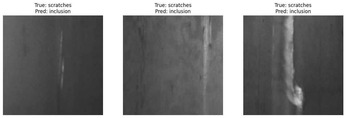
The image above shows the 3 mislabel images. Upon visual inspection, there are other factors which might confuse the model, like darker streaks through the image or a curved lighter area.
The code below saves any relevant information to be used in task 3.
Source
# generate df with misclassified images
misclassified_df = val_df.iloc[misclassified_indices].copy()
# add what it was misclassified as
misclassified_df['predicted_type'] = y_pred[misclassified_indices]
misclassified_df.to_csv('misclassified_images_2.csv', index=False)